Roll your own likelihood function with R

This document assumes you know something about maximum likelihood estimation. It helps you get going in terms of doing MLE in R. All through this, we will use the "ordinary least squares" (OLS) model (a.k.a. "linear regression" or "classical least squares" (CLS)) as the simplest possible example. Here are the formulae for the OLS likelihood, and the notation that I use.

There are two powerful optimisers in R: optim() and nlminb(). This note only uses optim(). You should also explore nlminb().

You might find it convenient to snarf a tarfile of all the .R programs involved in this page.

Writing the likelihood function

You have to write an R function which computes out the likelihood function. As always in R, this can be done in several different ways.

One issue is that of restrictions upon parameters. When the search algorithm is running, it may stumble upon nonsensical values - such as a sigma below 0 - and you do need to think about this. One traditional way to deal with this is to "transform the parameter space". As an example, for all positive values of sigma, log(sigma) ranges from -infinity to +infinity. So it's safe to do an unconstrained search using log(sigma) as the free parameter.

Here is the OLS likelihood, written in a few ways.

Confucius he said, when you write a likelihood function, do take the trouble of also writing it's gradient (the vector of first derivatives). You don't absolutely need it, but it's highly recommended. In my toy experiment, this seems to be merely a question of speed - using the analytical gradient makes the MLE go faster. But the OLS likelihood is unique and simple; it is globally quasiconcave and has a clear top. There could not be a simpler task for a maximisation routine. In more complex situations, numerical derivatives are known to give more unstable searches, while analytical derivatives give more reliable answers.

A simulation setup

To use the other files on this page, you need to take my simulation setup file.

Comparing these alternatives

Now that I've written the OLS likelihood function in a few ways, it's natural to ask: Do they all give the same answer? And, which is the fastest?

I wrote a simple R program in order to learn these things. This gives the result:

True theta =  2 4 6 
OLS theta =  2.004311 3.925572 6.188047 

Kick the tyres --
                 lf1() lf1() in logs    lf2()    lf3()
A weird theta 1864.956      1864.956 1864.956 1864.956
True theta    1766.418      1766.418 1766.418 1766.418
OLS theta     1765.589      1765.589 1765.589 1765.589
Cost (ms)        0.450         0.550    1.250    1.000

Derivatives -- first let me do numerically --
  Derivative in sigma     --  10.92756 
  Derivative in intercept -- -8.63967 
  Derivative in slope     -- -11.82872 
  Analytical derivative in sigma -- 10.92705 
  Analytical derivative in beta  -- -8.642051 -11.82950

This shows us that of the 4 ways of writing it, ols.lf1() is the fastest, and that there is a fair match between my claimed analytical gradient and numerical derivatives.

A minimal program which does the full MLE

Using this foundation, I can jump to a self-contained and minimal R program which does the full job. It gives this result:

True theta =  2 4 6 
OLS theta =  2.004311 3.925572 6.188047 

Gradient-free (constrained optimisation) --
$par
[1] 2.000304 3.925571 6.188048
$value
[1] 1765.588
$counts
function gradient 
      18       18 
$convergence
[1] 0
$message
[1] "CONVERGENCE: REL_REDUCTION_OF_F <= FACTR*EPSMCH"

Using the gradient (constrained optimisation) --
$par
[1] 2.000303 3.925571 6.188048
$value
[1] 1765.588
$counts
function gradient 
      18       18 
$convergence
[1] 0
$message
[1] "CONVERGENCE: REL_REDUCTION_OF_F <= FACTR*EPSMCH"

You say you want a covariance matrix?
MLE results --
          Coefficient  Std. Err.        t
Sigma        2.000303 0.08945629 22.36068
Intercept    3.925571 0.08792798 44.64530
X            6.188048 0.15377325 40.24138
Compare with the OLS results --
            Estimate Std. Error  t value      Pr(>|t|)
(Intercept) 3.925572 0.08801602 44.60065 7.912115e-240
X[, 2]      6.188047 0.15392722 40.20112 6.703474e-211

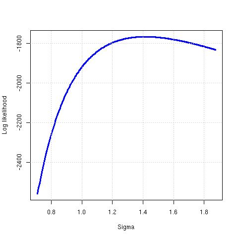
The file minimal.R also generates this picture:

Measurement about the full MLE

The R optim() function has many different paths to MLE. I wrote a simple R program in order to learn about these. This yields the result:

True theta =  2 4 6 
OLS theta =  2.004311 3.925572 6.188047 

                        Hit rate   Cost
L-BFGS-B, analytical         100   25.1
BFGS, analytical             100   33.1
Nelder-Mead, trans.          100   59.2
Nelder-Mead                  100   60.5
L-BFGS-B, numerical          100   61.2
BFGS, trans., numerical      100   68.5
BFGS, numerical              100   71.2
SANN                          99 4615.5
SANN, trans.                  96 4944.9

The algorithms compared above are:

L-BFGS-B, analytical. This uses L-BFGS-B which is a variant of BFGS which allows "box" constraints (you can specify a permitted range for each parameter). This uses the ols.gradient() function to do analytical derivatives. It is the fastest (25.1 milliseconds on my machine) and works 100% of the time.
BFGS, analytical. This uses BFGS instead of L-BFGS-B -- i.e. no constraints are permitted. Analytical derivatives are used.
Nelder-Mead, trans.. Nelder-Mead is a derivative-free algorithm. It does not need you to write the gradient. This variant uses the log() transformation in order to ensure that sigma is positive.
Nelder-Mead This is Nelder-Mead without the transformation.
L-BFGS-B, numerical This is the same L-BFGS-B but instead of giving him analytical derivative, I leave optim() to fend for himself with numerical derivatives. A worse than doubling of cost!
BFGS, trans., numerical This uses plain BFGS, with the log() transformation to ensure that sigma stays positive, but using numerical derivatives.
BFGS, numerical This is plain BFGS, with no transformation to ensure a sane sigma, and using numerical derivatives.
SANN This is a stochastic search algorithm based on simulated annealing. As you see, it failed for 1% of the runs. It is very costly. The attraction is that it might be more effective at finding global maxima and in "staying out of troublesome territory".
SANN trans. This uses the log() transform for sigma and does the search using simulated annealing.

Credits

I learned this with help from Douglas Bates and Spencer Graves, and by lurking on the r-help mailing list, thus learning from everyone who takes the trouble of writing there. Thanks!

Back up to my R knowledge base system

Ajay Shah
ajayshah at mayin dot org